
TL;DR
Cycle time is the actual time it takes to produce one unit while a process is running, calculated as net production time divided by the number of units made. It excludes downtime and planned stops, and the gap between ideal and actual cycle time is the speed loss that directly lowers the Performance factor of OEE.
Cycle time is the actual measured time it takes to produce one unit while the process is running. It is the heartbeat of a production line.
If a packaging machine completes one carton every 2.4 seconds, its cycle time is 2.4 seconds per unit. Crucially, cycle time only counts the time the equipment is actively running, so it excludes breakdowns, changeovers, and planned stops.
This is what makes cycle time different from broader timing metrics. It is a pure measure of process speed, not order fulfillment or scheduling. When cycle time drifts upward, your line is quietly making fewer parts per hour even when nothing has visibly broken, which is exactly why it is one of the most useful and most overlooked numbers on the floor.
The core formula is net production time divided by the number of units produced.
Cycle Time = Net Production Time / Number of Units Produced
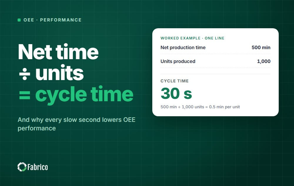
"Net production time" means the time the machine was actually running, with stops removed. If a line runs for 500 minutes of net production time and produces 1,000 units, the cycle time is 500 / 1,000 = 0.5 minutes, or 30 seconds per unit. This is the aggregate view, and it is the easiest to pull from production logs.
There is also a per-unit observed view, where you time individual cycles directly with a stopwatch or, more reliably, by reading the machine signal each time a part completes. The observed view exposes variation that the aggregate average hides: ten fast cycles and one very slow cycle can produce a healthy-looking average while masking a recurring stall.
Ideal cycle time is the fastest time per part your process can achieve on a sustained basis; actual cycle time is what it really achieves while running.
According to OEE.com, ideal cycle time is "the absolute fastest time per part that can be achieved by your manufacturing process on a sustained basis," while cycle time is "the actual measured time per part achieved by your manufacturing process while it is running."
The difference between the two is speed loss. You can quantify it directly:
Cycle Time Loss = Run Time - (Total Units x Ideal Cycle Time)
If actual cycle time ever appears faster than ideal, the ideal cycle time has been set wrong, usually overstated, and every downstream calculation built on it will be inaccurate. The ideal cycle time should come from the equipment manufacturer's rated speed or your best validated sustained run, not a hopeful guess.
| Term | What it measures | Set by | You control it? |
|---|---|---|---|
| Cycle time | Actual seconds/minutes to make one unit while running | Your process capability | Yes |
| Ideal cycle time | Fastest sustainable time per unit | Equipment rating | Benchmark only |
| Takt time | Required pace to meet customer demand | The market / orders | No |
| Lead time | Order placed to order delivered | Whole value stream | Indirectly |
Cycle time is the pace you actually hit, takt time is the pace you need to hit, and lead time is the total clock from order to delivery. These three are constantly confused, but they answer different questions.
Takt time is available production time divided by customer demand. It is the ceiling: if takt time is 60 seconds and your cycle time is 45 seconds, you are comfortably keeping up with demand. If cycle time climbs above takt time, you cannot meet orders without overtime or extra capacity.
Lead time is the longest of the three because it includes queueing, batching, and waiting, all the value-added and non-value-added time a customer experiences.
The healthy relationship is simple: cycle time should sit comfortably below takt time, and reducing cycle time creates the headroom that shortens lead time. We cover the demand-pacing side in depth in our guide to capacity utilization rate, so this article stays focused on the speed metric you directly own.
Cycle time is the entire engine behind the Performance factor of Overall Equipment Effectiveness. OEE has three factors, Availability, Performance, and Quality, and Performance is where every slow cycle and small stop shows up. The formula from OEE.com is:
Performance = (Ideal Cycle Time x Total Count) / Run Time
In other words, Performance compares how fast you could have run (ideal cycle time times every unit made) against how long the line was actually running. When actual cycle time creeps above ideal, the numerator shrinks relative to the denominator and Performance falls. This is why cycle time drift is so financially dangerous: it erodes OEE silently, without ever triggering a downtime alarm.
If you are building or auditing your OEE program, start with our complete guide to OEE and the step-by-step OEE calculation walkthrough. Slow cycles and small stops also map directly onto the six big losses framework, which categorizes exactly the speed losses cycle time exposes.
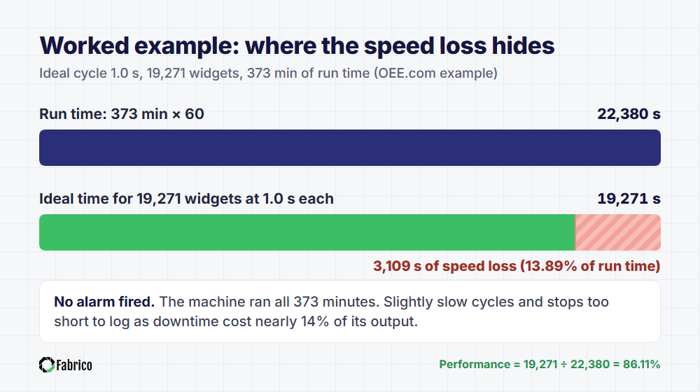
OEE.com's worked example makes the link concrete. With an ideal cycle time of 1.0 seconds, a total count of 19,271 widgets, and a run time of 373 minutes, Performance calculates as:
(1.0 second x 19,271 widgets) / (373 minutes x 60 seconds) = 0.8611, or 86.11%
That 13.89% gap is entirely speed loss. The machine ran the whole 373 minutes, but the cumulative effect of cycles running slightly slow, plus small stops too brief to log as downtime, cost nearly 14% of the line's potential output.
No alarm fired. That is the trap cycle time monitoring is built to close.
The fastest gains come from eliminating micro-stops and slow cycles, not from running equipment harder. Use this checklist as a starting point:
The common thread is visibility. Cycle time drift is invisible to the human eye because each lost fraction of a second is too small to notice. It only becomes visible when you measure every cycle and compare it to the ideal in real time.
Fabrico reads cycle times directly from machine PLCs, so drift surfaces the instant it starts rather than days later in a spreadsheet. Because Fabrico connects to the controller, it sees each completed part and the actual time it took, then compares that against the ideal cycle time automatically.
When cycles begin running slow, the Performance factor moves immediately and the cause is flagged, not buried in a monthly report. That cycle data feeds Fabrico's OEE software, which shows OEE live by line, machine and shift.
This matters because cycle time loss is a maintenance and process problem disguised as a speed problem.
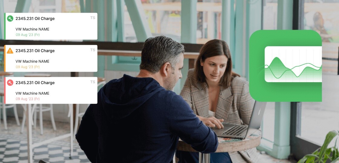
When Fabrico's live cycle data shows a slowdown, the operator tags the cause on a tablet and a technician can open a digital work order for that machine on a phone, taking a slow cycle through to a confirmed fix.
Tying real-time cycle data to the repair work is how a plant stops silent speed loss from quietly eroding OEE. Fabrico is built in the EU and hosted on AWS in an EU region.
If you want to see real-time cycle-time capture and the work order flow on your own lines, book a Fabrico demo.
Setting the standard behind that cycle time? Our time study data model covers the observation sheet fields, ratings and allowances.
Slow cycles are the performance loss in OEE. The cost of downtime calculator puts a yearly price on the gap between your current OEE and the OEE you could reach.
The core formula is net production time divided by the number of units produced. If a line runs 500 minutes of net production time and makes 1,000 units, cycle time is 500 / 1,000 = 0.5 minutes, or 30 seconds per unit. Net production time excludes downtime and planned stops, so cycle time reflects only the speed of the process while it is actively running.
Ideal cycle time is the fastest time per part your process can achieve on a sustained basis, usually set from the equipment's rated speed. Actual cycle time is what the process really achieves while running. The gap between them is speed loss.
If actual cycle time ever appears faster than ideal, the ideal cycle time has been set incorrectly and should be corrected, because every OEE calculation built on it will be inaccurate.
Cycle time drives the Performance factor of OEE. The formula is Performance = (Ideal Cycle Time x Total Count) / Run Time. When actual cycle time creeps above ideal, the line makes fewer parts per running minute, the numerator shrinks relative to run time, and Performance falls.
Slow cycles and small stops both show up here, which is why cycle time drift can erode OEE without ever triggering a downtime alarm.
Cycle time is the pace your line actually hits, measured on the floor. Takt time is the pace you need to hit to meet customer demand, calculated as available production time divided by demand. Takt time is the ceiling set by the market, while cycle time is the capability you control.
A healthy line keeps cycle time comfortably below takt time so it can meet orders without overtime or extra capacity.
The fastest gains come from eliminating small stops and slow cycles rather than running equipment harder. Measure the per-unit cycle instead of only the shift average, hunt micro-stops like jams and misfeeds, validate the ideal cycle time benchmark, reduce changeover variation with SMED, standardize operator method across shifts, and address tooling and lubrication drift early through preventive maintenance. The common requirement is real-time visibility into every cycle.
Cycle time drift is invisible to the human eye because each lost fraction of a second is too small to notice, and manual logs only surface the problem days later as an average.
Reading cycle times directly from machine PLCs captures every completed part and compares it to the ideal cycle time instantly, so the Performance factor moves the moment drift starts and the cause can be flagged and fixed before it erodes OEE for an entire shift.
Related: reduce manufacturing lead time, compressing the full order-to-delivery window, not just the machine cycle.
See how Fabrico unifies OEE and maintenance in one platform.
Request a demo









 Login
Login
 Blog
Blog