


 Login
 Blog

Cellular Manufacturing: Layout, Examples and When a Cell Pays Off

In short: Cellular manufacturing groups the machines and people needed to make one family of similar parts into a small, self-contained cell, usually U-shaped, so each part moves from step to step one piece at a time instead of queuing in batches between departments. The result is shorter lead times, less work in process and faster feedback on quality.
- A cell is built around a part family: products with similar routings.
- Removing buffers couples the stations. A stop at any one of them stops the whole cell, so cell availability is the product of station availabilities.
- A cell pays off when its OEE stays above demand / ideal output with headroom. Check that before you move a single machine.
Guide, updated 14 November 2026. Sources are listed at the end.
What is cellular manufacturing?
Cellular manufacturing is a lean layout method. The US Environmental Protection Agency's lean methods guide on cellular manufacturing describes it as arranging production work stations and equipment in a sequence that supports smooth flow, with minimal transport or delay. Products move through the cell one piece at a time, at a rate set by customer demand, instead of in batches that wait in front of each department.
The idea comes from group technology: sort the products into part families with similar processing needs, then give each family its own cluster of machines. A review from the University of South Australia, presented to the Production and Operations Management Society, puts it the same way: operators process part families in cells, or clusters of dedicated machines that may be dissimilar in function. A saw, a lathe, a mill and a deburring station sit next to each other because one family of parts visits them in that order.
The cellular manufacturing system in practice
- Part family: the products the cell makes. They share their main process steps in the same order, and changeovers between them are short.
- Dedicated equipment: the machines the family needs, often smaller and simpler than shared department machines. EPA's guide notes a rule of thumb that machines need not be more than three times larger than the part they make.
- Cross-trained team: operators run several machines and move with the work. EPA describes the shift from watching one machine to managing several.
- Flow at demand rate: parts enter the cell as customer demand pulls them, and the cell's pace follows line balancing of the work across the stations.
- Little or no work in process between stations: one piece, or a very small batch, moves at a time.
Cellular manufacturing layout
A cell is usually laid out in a U or C shape. EPA's guide says machines are placed close together in a U or C to cut the operator's movement, with only a minimal amount of work in process, and that the flow often runs counterclockwise to suit right-handed movements. The U puts the first and last steps side by side, so one operator can load a new part and unload a finished one in the same walk, and it lets the team add or remove operators as demand changes.
Cell, functional layout or flow line?
| Functional (process) layout | Cellular layout | Dedicated flow line | |
|---|---|---|---|
| Grouped by | Machine type: all lathes together | Part family: the machines one family needs | One product or a few variants |
| Product mix | High mix, any routing | Medium mix within a family | Low mix, high volume |
| Work in process | High: batches queue at every department | Low: one piece or small batches | Low, set by conveyor and buffers |
| Lead time | Days to weeks | Hours to a day | Hours |
| Stations coupled? | No, buffers decouple them | Yes, a stop anywhere stops the cell | Yes, unless buffers are designed in |
| Operators | One machine each, specialists | Several machines each, cross-trained | Fixed stations |
| Main risk | Long lead times, lost parts, late quality feedback | One weak station caps the whole cell | Inflexible when the product changes |
Benefits of cellular manufacturing, with the numbers
The benefits come mainly from removing queues. Little's Law makes that exact. In his 2011 review in Operations Research, John D. C. Little gives the operations management form of the law: throughput = work in process / cycle time, where cycle time is the time a part spends in the system. Rearranged, WIP = throughput x lead time. Keep output the same, cut lead time from 8 days to 1, and work in process falls to an eighth. Little notes the corollary for managers: more output needs more WIP or a shorter cycle time, unless the process itself changes.
A real case shows the size of the change. A NIST Manufacturing Extension Partnership success story describes Current Applications, an electric motor maker in Watertown, New York, with about 60 employees. With help from its MEP centre it built one-piece flow cells in two product lines and balanced the work with work balance charts. Lead time fell 50%, work in process fell from 105 units to 5, output rose from 40 to 105 units a day, and a 1,000-unit backlog was cleared.
The UniSA review lists the usual benefits from the research literature: shorter setup times, less material handling, less work in process, shorter cycle times and lower tooling needs, along with better quality and space use. It also notes that cells were adopted by between 43% and 53% of firms in the US and the UK in one study, and that firms converting to cells often struggle and get less than they expected, with people issues such as training, communication and teamwork a frequent cause. EPA adds environmental gains: less overproduction, fewer defects because problems surface quickly, and less floor space to heat, cool and light.
The hidden cost: coupled stations
Buffers between departments do a quiet job. When the mill breaks down in a functional layout, the lathe keeps working into the queue, and the deburr station keeps working off its own queue. Take the buffers away and the stations become one system. When any station stops, the whole cell stops.
Reliability engineers call this a series system. The NIST/SEMATECH e-Handbook's series model states the rule: in a series model, multiply reliabilities. The system fails when the first component fails. Applied to availability, a cell of four stations that are each available 95% of the time is available about 0.95 x 0.95 x 0.95 x 0.95 = 81.5% of the time, if their stops do not overlap. Eight such stations give 66.3%.
That is the trade a cell makes: much less work in process and lead time, for a whole that is only as available as the product of its parts. It is why EPA's guide pairs cells with quick changeover, autonomation and total productive maintenance, and why the step after building a cell is measuring it.
Worked example: a machining cell, in OEE and money
Example data. All figures below are assumptions for a typical machine shop, except the margin and the interest rate, which are sourced as marked.
The money starts from one sample input, set before any result: a selling price of $60 a valve body. The margin comes from NYU Stern's margin dataset by industry (Aswath Damodaran, January 2026 data, accessed 15 November 2026), which reports a gross margin of 37.47% for 105 US machinery firms. So each part contributes about $60 x 37.47% = $22.48, and a part in process is worth its cost, $60 x (1 - 0.3747) = $37.52. Gross margin is a cautious stand-in for contribution, because it still carries fixed plant cost.
Before: a functional layout
A shop makes a family of valve bodies through four steps: saw, CNC lathe, CNC mill, deburr and wash. Demand is 600 parts a day. In the functional layout the parts travel in batches between departments, and the average part spends 8 days in the shop. By Little's Law, work in process = 600 x 8 = 4,800 parts. At $37.52 a part in process, that is 4,800 x $37.52 = $180,096 of cash on the floor.
After: a U-shaped cell
The four machines move into a U-shaped cell run by a cross-trained team. Lead time falls to 1 day, so work in process = 600 x 1 = 600 parts, or 600 x $37.52 = $22,512. The cell frees $180,096 - $22,512 = $157,584 of working capital. At the 7.00% bank prime loan rate in the Federal Reserve's H.15 release of 13 November 2026, the interest on that cash alone is $157,584 x 0.07 = $11,030.88 a year, before any saving in space, handling or scrap.
The cell's OEE
The mill is the slowest machine, with an ideal cycle of 60 seconds a part, so it sets the cell's pace. Two shifts of 7.5 planned hours give 2 x 27,000 seconds / 60 = 900 parts a day of ideal output.
- Station availability: saw 98%, lathe 96%, mill 95%, deburr and wash 97%.
- Cell availability: 0.98 x 0.96 x 0.95 x 0.97 = 86.7%.
- Performance 92% (short stops and the cell running below ideal pace), quality 98%.
- Cell OEE: 0.867 x 0.92 x 0.98 = 78.2%, or about 703 good parts a day of capacity.
In the old functional layout, the mill's own availability of 95% set the limit, because buffers protected it from the other stations. Its OEE was 0.95 x 0.92 x 0.98 = 85.7%. The cell gave up 7.5 points of OEE, about 67 parts a day, in exchange for the cash and the lead time. With demand at 600, the cell can afford it.
The rule for when a cell pays off
The test is one line:
Required cell OEE = demand / ideal output. The cell works if its real OEE is above that, with headroom for bad weeks.
Here, required OEE = 600 / 900 = 66.7%. Actual cell OEE is 78.2%, so there are 11.5 points of headroom. Now suppose demand grows to 750 parts a day. Required OEE becomes 750 / 900 = 83.3%, above what the cell can do. The shop has three choices: raise station availability, add a small buffer before the weakest station, or add overtime.
Raising the mill's availability from 95% to 98%, for example by cutting its tool changes and setups, lifts cell availability to 0.98 x 0.96 x 0.98 x 0.97 = 89.4% and cell OEE to 80.6%. That is 900 x (0.806 - 0.782) = about 22 more good parts a day. At the $22.48 each part contributes and 250 working days, that is 22 x $22.48 x 250 = $123,640 a year once demand is there to take it. In a cell, one station's downtime is the whole cell's downtime, so a fix on the weakest station pays for the whole cell.
Book a demo and see OEE and losses per line and shift.
When cellular manufacturing fits, and when it doesn't
Use the rule above, plus these checks, before you move machines:
- A real part family exists. The products share their main steps in the same order. If every part has a different routing, a cell becomes a small job shop with the same queues.
- Demand is steady enough to keep the cell loaded. A cell that sits idle half the week ties up machines that a functional layout would share.
- Changeovers inside the family are short. One-piece flow with long setups turns into batch flow again.
- Station availability is high. If the product of availabilities is below the required OEE, fix reliability first, or keep a small buffer at the weakest station.
- Machines can be dedicated or duplicated. A single expensive machine that every family needs cannot sit in one cell. Leave it as a shared monument and design the cells around it.
- People are ready. Cross-training, a team leader and a pay system that does not reward one-machine output. The UniSA review points to these social factors as a common reason cells disappoint.
Cellular manufacturing examples
- Machining: a saw, lathe, mill and deburr cell for a family of shafts or valve bodies, as in the worked example.
- Electric motor assembly: the NIST MEP case above, where one-piece flow cells cut work in process from 105 units to 5.
- Electronics: a cell that places, solders, tests and packs one board family, with operators moving between stations.
- Fabrication: cutting, bending and welding for one family of brackets or frames, laid out in a U so material enters and leaves at one end.
- Assembly and kitting: manual stations in a U with parts presented at the point of use, paced to demand. The same logic underlies one-piece flow.
How to set up a manufacturing cell, step by step
- Measure the current state. EPA's first step: product and process data, value stream maps, cycle times and lead times, and which equipment can move. Record work in process and OEE of each machine, so you have a baseline.
- Find the part family. Group products by routing. A product-routing matrix in a spreadsheet often shows the families quickly.
- Size the cell. Ideal output = planned time / bottleneck cycle time. Required OEE = demand / ideal output. Multiply the station availabilities you measured and check you have headroom.
- Design the layout. U or C shape, first and last steps together, machines close, material presented at the point of use.
- Balance the work across operators to the demand rate, and write standard work.
- Move, test and train. Run trial parts, fix what breaks, and train the team on every station.
- Measure the cell as one unit. Track cell OEE, the downtime of each station and the reasons, every shift.
- Improve the weakest station first, with quick changeover, maintenance and root cause work.
Common mistakes
- Measuring each machine's OEE but not the cell's. Four machines at 90% can still make a cell that misses demand. The cell's output is the number that matters.
- Removing every buffer at once. Start with small, fixed buffers at the least reliable station, then shrink them as availability improves.
- Building a cell around a family that isn't one. If a third of the parts skip a station or need an outside step, the flow breaks.
- Ignoring the people side. Cells need cross-training, shared targets and a team leader. Without them, operators guard their own machine as before.
- Moving machines without a baseline. If you don't record lead time, WIP and OEE before, you cannot prove the cell worked, or spot that it didn't.
- Forgetting the shared machines. A heat treatment or plating step outside the cell can bring back the queues you removed.
For plant, production and CI managers
This week
- Pull routings for your top 50 parts by volume and sort them into families by sequence of operations.
- For one candidate family, measure today's lead time and work in process. Little's Law gives one from the other if you know daily output.
- Collect the availability of each machine the family uses, from logs or a two-week manual record.
- Multiply them and compare with demand / ideal output. That tells you whether a cell would work today or needs reliability work first.
This quarter
- Fix the weakest station's availability before the move: setups, tooling, maintenance.
- Build one pilot cell, with a small buffer at the weakest station.
- Track cell OEE and station stops by reason every shift, and review weekly with the team.
- Cut the buffer as availability rises, and record the WIP and lead time each month.
- Put the result in money: cash freed from WIP, interest saved, and output gained per point of cell OEE. Then choose the next family.
Measuring a cell as one unit is where OEE software earns its keep: it shows the cell's OEE and which station stopped it, shift by shift. A light MES adds the orders and products running through the cell, so changeovers within the family show up in the data.
How Fabrico fits
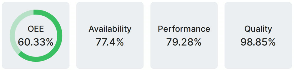
Fabrico is a cloud OEE and light MES platform. It shows OEE and losses by machine, line and shift, from the PLC or a Fabrico IoT device, with the reasons operators add on a tablet or phone. For a cell, that means the cell's OEE next to the stops of each station.
On manual stations, AI cameras (an add-on) count output.
Book a demo and see downtime per line and shift.
What people ask next
What is a cellular manufacturing system?
It is a way of organising production in which the machines and people needed for one family of similar parts are grouped into a small cell. Parts move from step to step one piece at a time at the rate of demand, instead of queuing in batches between departments.
What does a cellular manufacturing layout look like?
Usually a U or C shape, with the machines close together and the first and last steps side by side. Operators work inside the U and run several machines, and there is little or no work in process between stations.
What are examples of cellular manufacturing?
A saw, lathe, mill and deburr cell for a family of machined parts; one-piece flow cells for electric motor assembly; a place, solder, test and pack cell for one board family; and cut, bend and weld cells for brackets or frames.
What are the benefits of cellular manufacturing?
Shorter lead times, less work in process, less material handling and faster quality feedback. By Little's Law, cutting lead time from 8 days to 1 at the same output cuts work in process to an eighth.
What are the disadvantages of cellular manufacturing?
Removing buffers couples the stations, so a stop at any one stops the cell and cell availability is the product of station availabilities. Cells also need a real part family, steady demand, short changeovers and cross-trained people.
How do you calculate OEE for a manufacturing cell?
Measure the cell as one unit: good parts out of the cell x the bottleneck's ideal cycle time / planned time. To check a design, multiply the station availabilities, then multiply by performance and quality, and compare with demand / ideal output.
Sources
All sources accessed on 14 November 2026, except those marked as accessed on 15 November 2026. Dates are the publication dates shown on each page.
- NIST/SEMATECH e-Handbook of Statistical Methods, 8.1.8.2 Series model, undated, accessed 14 November 2026
- US Environmental Protection Agency, Lean Thinking and Methods: Cellular Manufacturing, last updated 16 March 2026
- NIST Manufacturing Extension Partnership, Lean Tools Provide Lead Time Reduction (Current Applications, Watertown, NY), 2024 success story, accessed 14 November 2026
- John D. C. Little, Little's Law as Viewed on Its 50th Anniversary, Operations Research 59(3), 536-549, 2011
- Fraser, Harris and Luong, University of South Australia, Team-based cellular manufacturing: a review and survey to identify important social factors, POMS conference paper 004-0331, 2006
- Federal Reserve Board, H.15 Selected Interest Rates (bank prime loan), 13 November 2026
- NYU Stern, Aswath Damodaran, Operating and Net Margins by Industry (US), Machinery row, January 2026 data, accessed 15 November 2026
Related articles


Latest from our blog



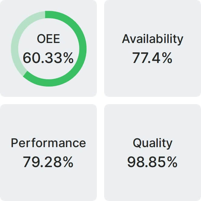
Real Fabrico tiles, sample data.