


 Login
 Blog

Economies of Scale in Manufacturing: Examples, Limits and the Scale You Already Own

In short: Economies of scale in manufacturing are the fall in cost per unit as a plant or company makes more. Fixed costs such as equipment, buildings and crews are spread over more units, bigger equipment costs less per unit of capacity, and larger buyers pay less for inputs. Past a point, costs per unit rise again: these are diseconomies of scale.
- The lowest point of the long-run cost curve is the minimum efficient scale. Bigger than that brings little or no saving.
- Capital cost grows more slowly than capacity: under the six-tenths rule, twice the capacity costs about 1.52 times as much.
- The cheapest scale economy is often the plant you already have: more good output from the same fixed cost lowers cost per unit without new capital.
Guide, updated 14 November 2026. Sources are listed at the end.
What are economies of scale in manufacturing?
The open economics textbook OpenStax Principles of Economics (2e), section 7.5 defines economies of scale simply: as the quantity of output goes up, the cost per unit goes down. Its example is an alarm clock maker. A small factory makes 1,000 clocks at $12 each, a medium one 2,000 at $8 each, and a large one 5,000 at $4 each. Same product, a third of the unit cost.
In a plant, that pattern has two different sources, and mixing them up leads to expensive decisions:
- Scale you buy: a bigger plant, a faster line, a larger furnace. The cost curve itself moves down, and the investment is large.
- Scale you already own: more good output from the line you have. Fixed costs stay the same and are spread over more units. The investment is small, and the result shows up directly in OEE cost per unit.
Economists draw the first on the long-run average cost curve and the second on a short-run curve for a given plant. Plant managers live mostly on the second, and finance teams tend to propose the first. This guide covers both and shows how to compare them in money.
Where the savings come from
Economies of scale in manufacturing have a handful of practical sources:
- Spreading fixed costs. Depreciation, rent, supervision, base-load energy and much of the crew cost do not change with each unit made. More units per year means less fixed cost in each.
- Cheaper capacity. Larger equipment usually costs less per unit of capacity. A tank twice the volume does not need twice the steel. The six-tenths rule below puts numbers on it.
- Specialisation. Higher volume justifies dedicated lines, fixtures and people, with fewer changeovers per unit.
- Purchasing. Larger orders get better prices and lower handling cost per unit.
- Spreading overheads across the company. Engineering, quality systems, IT and sales cost about the same whether they support one plant or three.
The first source is available to every plant, at any size, every day. The others need volume that the market will buy.
How concentrated scale is in practice
US data shows how much output sits in large plants, and how many small plants still thrive. The US Census Bureau's Annual Survey of Manufactures methodology notes that the recent Economic Censuses contained about 290,000 active manufacturing establishments. About 17,000 of them, selected with certainty because of their size (one criterion is 1,000 or more employees), accounted for approximately 70% of the total value of shipments in the 2017 Economic Census.
At the same time, a Census Bureau analysis of 2015 County Business Patterns data found that establishments with 1,000 or more employees were 0.3% of manufacturing establishments but employed over 15% of manufacturing workers. In cement and concrete products, 92% of establishments had fewer than 50 employees. Scale wins in some industries and not in others, which is where minimum efficient scale comes in.
Minimum efficient scale and the long-run cost curve
OpenStax builds the long-run average cost curve from a family of short-run curves, one for each plant size, and takes the lowest cost available at each output. A typical curve has three parts:
- Economies of scale: the curve falls. Bigger is cheaper per unit.
- Constant returns to scale: the curve is flat. Once the economies are used up, growing all inputs together barely changes average cost.
- Diseconomies of scale: the curve rises. Bigger becomes dearer per unit.
The output where the curve first reaches its lowest point is called the minimum efficient scale. OpenStax shows why it matters with a dishwasher example: a market of 1 million dishwashers a year, and a cost curve whose lowest point is at 10,000 units. That market supports about 100 plants at the efficient size. If the flat bottom runs from 5,000 to 20,000 units, there is room for anywhere from 50 to 200 producers. If total demand were only 30,000, about three firms would compete; at 5,000, a single producer is the likely outcome.
For a manufacturer, the lesson is that a plant below minimum efficient scale fights a structural cost gap, while a plant on the flat part gains little from getting bigger. On the flat part, the money is in running the existing capacity well.
Diseconomies of scale
Costs per unit eventually rise with size. OpenStax names the main causes: factories become hard to manage, many layers of management slow communication, and communication failures disrupt the flow of work and materials. It also describes a firm-wide version it calls the leviathan effect.
On the shop floor, diseconomies look familiar:
- A large line where one stop halts everything, so availability falls as the line gets longer and more coupled.
- Longer internal transport and larger work in progress between departments.
- Decisions about a stopped machine that wait for someone two levels up.
- Product variety added to fill a large plant, with more changeovers per unit as a result.
- Outbound freight: a single big plant ships further to reach the same customers.
None of these show up in a capital cost estimate. All of them show up in OEE, which is one reason to measure OEE before and after any expansion.
The six-tenths rule: how capital cost scales
Engineers estimate the cost of bigger equipment with a cost-capacity equation. The open textbook Foundations of Chemical and Biological Engineering I (Verret, Qiao and Barghout, BCcampus) writes it as:
Ca / Cb = (Aa / Ab)n
where C is cost, A is capacity and n is the cost exponent. It notes a general rule, the six-tenths rule: for many processes the exponent is close to 0.60.
With n = 0.6, doubling capacity multiplies the cost by 20.6 = 1.52. Capital per unit of capacity falls to 1.52 / 2 = 0.76 of the original, a 24% saving. That is the classic engineering source of economies of scale.
The exponent varies by equipment. The textbook's table gives 0.85 for a multi-stage air compressor, 0.60 for a stainless shell-and-tube heat exchanger, 0.67 for a stainless centrifugal pump, 0.47 for a crystallizer and 0.30 for a carbon steel horizontal tank. Its worked example shows the difference: a 0.8 m3 crystallizer costing $35,000 scales to about $65,100 at 3.0 m3 with the table exponent, and about $77,400 with the six-tenths rule.
Two cautions for manufacturers. First, the rule describes equipment cost, not running cost; a line twice the size still needs crews, energy and materials. Second, the saving per unit only arrives if the larger capacity is sold and run. A big line at low utilisation has a higher cost per unit than a small line running full.
Worked example: scale you own vs scale you buy
Example data. A plant runs one packing line. The costs below use published unit prices where marked; the line size, crew and capital are assumptions.
The line's fixed costs
- Planned time: two 8-hour shifts on 250 days, 4,000 hours a year. Example data.
- Crew: 6 people per shift. Labour cost: $37.21 an hour in total compensation, or $25.03 in wages only, for private industry production occupations in June 2026, from the BLS Employer Costs for Employee Compensation, Table 4. 4,000 x 6 x $37.21 = $893,040 a year ($600,720 at wages only).
- Base-load power: 150 kW whenever the line is planned to run (example data), at 9.64 cents per kWh, the US industrial average for August 2026 in the EIA's Electric Power Monthly, Table 5.6.A. 600,000 kWh x $0.0964 = $57,840 a year.
- Depreciation: a $3.0 million line over 10 years, $300,000 a year. Example data.
Total fixed cost: $893,040 + $57,840 + $300,000 = $1,250,880 a year ($958,560 counting wages only). The line's ideal output is 3,000 units an hour, or 12 million units a year in planned time. Example data.
Scale you already own
Fixed cost per unit depends on how much of that ideal output the line actually delivers as good units. For a realistic baseline, use the Federal Reserve's G.17 release of 16 October 2026: US manufacturing capacity utilisation was 75.9% in September 2026, 2.3 points below its 1972 to 2025 average of 78.2%. Capacity utilisation is a national measure, not OEE, but it is a fair, sourced range for how full an average plant runs.
| Share of ideal output | Good units a year | Fixed cost per unit (total comp) | Fixed cost per unit (wages only) |
|---|---|---|---|
| 75.9% (US, September 2026) | 9,108,000 | 13.73 cents | 10.52 cents |
| 78.2% (US average, 1972 to 2025) | 9,384,000 | 13.33 cents | 10.21 cents |
Moving from 75.9% to 78.2% adds 276,000 good units with no new fixed cost. Fixed cost per unit falls by 2.94%. On 9,384,000 units, that is $28,193 to $36,791 a year on one line, depending on whether you count wages only or full compensation. Each further point near that level is worth about $12,300 to $16,000 a year.
These are modest numbers on purpose: they come from the gap between today's national rate and its long-run average, not from an assumed jump. Plants that run well below the national rate, or that have several lines, multiply them. The mechanism is the same one OpenStax uses for its alarm clocks, without building a new factory.
Scale you buy
Now suppose the plant considers a second line with twice the capacity. Under the six-tenths rule, it costs about $3.0 million x 1.52 = $4.55 million, not $6.0 million. If both lines ran at the same 75.9%, depreciation per unit would fall from 3.29 cents on the existing line to 2.50 cents on the new one. That is a real economy of scale, but it depends on three conditions:
- The market buys 18.2 million more units a year at 75.9% utilisation.
- The bigger line holds the same utilisation. Longer, more coupled lines can lose availability to the diseconomies listed above.
- The crew, energy and materials per unit do not rise with the size of the line.
If any one fails, the capital per unit saving shrinks or disappears, while the $4.55 million is spent either way. The existing line's 2.3 points, by contrast, need no capital and carry no market risk. That is why the order matters: recover the capacity you own, then size new capacity on the volume you still cannot make. For a fuller comparison, see new production line cost vs recovering capacity.
Book a demo and see OEE and losses per machine and shift.
Economies of scale vs related ideas
| Idea | What lowers cost per unit | Needs new capital? | Where it shows |
|---|---|---|---|
| Economies of scale (plant size) | A bigger plant or line on a lower cost curve | Yes | Long-run average cost curve |
| Fixed-cost spreading (utilisation) | More good output from the same plant | Little or none | OEE, capacity utilisation, cost per unit |
| Learning curve | Experience: fewer hours per unit as cumulative output grows | No | Hours or cost per unit vs cumulative units |
| Economies of scope | Sharing assets across several products | Sometimes | Cost of a product range vs separate plants |
| Diseconomies of scale | Nothing: cost per unit rises with size | Comes with growth | Coordination losses, longer lines, freight |
Learning and scale are often confused because both lower cost as volume grows. Learning depends on cumulative output over time; scale depends on the rate of output and the size of the plant. A plant can have one without the other.
Common mistakes
- Assuming bigger is always cheaper. Past minimum efficient scale, the curve is flat or rising. Check which part of the curve you are on.
- Applying the six-tenths rule to everything. The exponent ranges from 0.30 to 0.85 across the textbook's equipment table. Use the exponent for the equipment in question when you have it.
- Counting capacity as output. Unit cost savings depend on good units sold, not nameplate capacity. A bigger line running half full is a dearer line.
- Ignoring the plant you have. Two or three points of utilisation on existing lines can cost far less than an expansion and carry no market risk.
- Leaving diseconomies out of the business case. Longer lines, more variety and more layers cost money too. Put an availability assumption in the case and test it against today's lines.
- Treating labour as fully variable. In many plants the crew is paid for the shift, not per unit. That makes labour part of the fixed cost that more output spreads.
- Confusing scale with learning. A drop in cost per unit after launch may be learning, not scale. The fixes differ.
For plant, production and CI managers
Expansion decisions usually start in finance or sales. The facts that should drive them sit on the shop floor.
This week
- List the fixed costs of your highest-volume line for a year: crew per shift, base-load energy, depreciation, supervision.
- Divide them by last year's good units to get fixed cost per unit. Then divide by the units at ideal rate over planned time. The gap between the two figures is what lost output costs you.
- Compare your line's share of ideal output with the national rate of 75.9% and the long-run average of 78.2%. Where does it sit?
- Price one point of extra output on that line, the way the worked example does.
This quarter
- Before any capacity request goes to the board, show the capacity already lost on existing lines in units and money, by loss type. Read more on capacity utilisation to set the baseline.
- For any new line, put the six-tenths estimate next to an honest utilisation assumption, taken from the existing lines' measured output, not from the vendor's nameplate.
- Add diseconomy risks to the case: longer coupled lines, more changeovers, extra transport. Price each one with today's OEE data.
- Pick the largest loss on the main line and run one improvement project on it. Track the change in good units and fixed cost per unit.
- Recalculate fixed cost per unit every quarter, so the effect of better running is visible to finance.
Good units from the existing plant are the raw material for every number above. OEE software records counts, run time and stops per machine and shift automatically, and a light MES ties them to orders and products, so fixed cost per unit can be tracked by line and product.
How Fabrico fits
Fabrico is a cloud OEE and light MES platform. It shows OEE and losses by machine, line and shift, from the PLC or a Fabrico IoT device, with the reasons operators add on a tablet or phone. That gives you good units and lost capacity per line, the two numbers that decide whether to run the plant fuller or build a bigger one.
On manual stations, AI cameras (an add-on) count output.
Book a demo and see good output per line and shift.
What people ask next
Should I build a bigger line or run my current lines fuller?
Run the current lines fuller first. More good output from the same fixed cost lowers cost per unit with little capital and no market risk. Size new capacity on the volume you still cannot make once existing losses are recovered.
How much cheaper per unit is a line with twice the capacity?
Under the six-tenths rule, twice the capacity costs about 1.52 times as much, so capital per unit of capacity falls by about 24%. The exponent varies by equipment, from 0.30 to 0.85 in one textbook table, and the saving only arrives if the larger line is sold and run.
How do I know if my plant is past its minimum efficient scale?
Minimum efficient scale is the output where long-run average cost first reaches its lowest point. If cost per unit stopped falling as volume grew, or coordination, changeovers and transport are rising faster than volume, you are on the flat or rising part of the curve.
What causes diseconomies of scale in a factory?
Management layers that slow decisions, communication failures that disrupt the flow of work and materials, long coupled lines where one stop halts everything, extra product variety and longer freight. They show up as lost availability and higher overhead per unit.
How much is one point of extra output worth on my line?
Divide the line's yearly fixed cost by its good units before and after. In the worked example, a line with about $1.25 million of fixed cost a year gains $12,300 to $16,000 a year per point near 78% of ideal output, using BLS labour and EIA power prices.
Is labour a fixed or variable cost when I calculate cost per unit?
In many plants the crew is paid for the shift, not per unit, so crew labour behaves like a fixed cost that more good output spreads. Treat it as variable only where staffing really moves with volume.
Sources
All sources accessed on 14 November 2026. Dates are the publication dates shown on each page.
- OpenStax, Principles of Economics 2e, 7.5 Costs in the Long Run (Rice University), undated, accessed 14 November 2026
- Verret, Qiao and Barghout, Foundations of Chemical and Biological Engineering I, 6.2 Purchased Equipment (PE) Cost (BCcampus, Engineering LibreTexts), undated, accessed 14 November 2026
- Federal Reserve Board, G.17 Industrial Production and Capacity Utilization, 16 October 2026
- US Census Bureau, Annual Survey of Manufactures: Methodology, undated, accessed 14 November 2026
- US Census Bureau, Small Manufacturers Play a Big Role in the U.S. Economy, 16 November 2017
- US Bureau of Labor Statistics, Employer Costs for Employee Compensation, Table 4, June 2026, 9 September 2026
- US Energy Information Administration, Electric Power Monthly, Table 5.6.A, 23 October 2026
Related articles












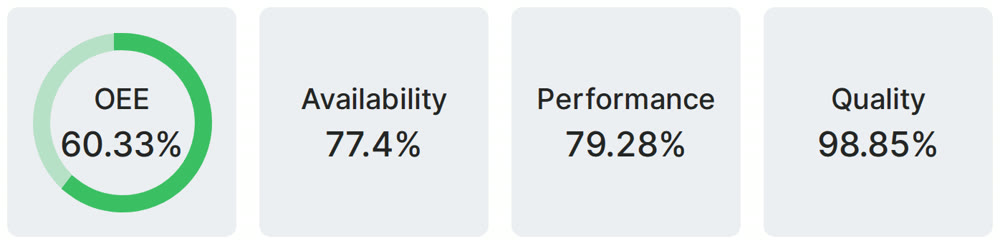
Real Fabrico tiles, sample data.