


 Login
 Blog

Learning Curve in Manufacturing: Formula, Wright's Law and a Ramp-Up Example

In short: The learning curve in manufacturing says that the labour, time or cost needed to make one unit falls by a steady percentage each time cumulative output doubles. On an 80% learning curve, unit 2 takes 80% of the time of unit 1, unit 4 takes 80% of unit 2, and so on. T. P. Wright described it for aircraft in 1936, which is why it is also called Wright's law.
- Formula: Y = A x Xb, where A is the first unit's hours or cost, X the unit number and b = ln(slope) / ln 2.
- The slope is not a constant of nature. Measure it from the plant's production data and manage it like any other rate.
- Production breaks erase part of the learning. Price that loss before you plan a shutdown or move a crew.
Guide, updated 14 November 2026. Sources are listed at the end.
What is the learning curve in manufacturing?
A learning curve describes how the effort to make a product falls as the plant makes more of it. People find faster methods, supervisors fix the awkward steps, tools get adjusted and the paperwork settles down. The first unit of a new product is slow and expensive. The hundredth is much cheaper. The thousandth is cheaper again, but the gain per unit is smaller.
The idea comes from aircraft production. The US Government Accountability Office's Cost Estimating and Assessment Guide (GAO-20-195G) credits T. P. Wright with starting the discussion in 1936, in a paper called "Factors Affecting the Cost of Airplanes". Wright saw that labour per airframe fell by a near-constant share each time the number of airframes built doubled. Government cost estimators still use it, and GAO's guide sets out the method in its Appendix VII.
Three terms cover the same pattern:
- Learning curve: the usual name in operations and cost estimating, mostly applied to labour hours per unit.
- Wright's law: the name used when the idea is applied to whole technologies, such as solar panels or batteries.
- Experience curve: a wider version that covers total unit cost, including materials and overhead, not only labour.
For a plant manager the practical question is simple: how many hours will unit 50, unit 500 or unit 5,000 take, and what will the ramp-up cost before the line reaches its standard?
The learning curve formula
GAO's unit formulation page writes the curve as:
Y = A x Xb
- Y is the hours or cost of unit number X.
- A is the hours or cost of the first unit (cost estimators call it T1).
- X is the unit number.
- b is the slope coefficient: b = ln(slope) / ln 2. For an 80% curve, b = ln 0.8 / ln 2 = minus 0.322.
GAO's own example uses a first unit of $1,000 and an 80% curve. Unit 2 costs $1,000 x 2-0.322 = $800, unit 3 costs $702 and unit 4 costs $640. The cost falls by the slope every time the quantity doubles: $1,000, then $800 at unit 2, then $640 at unit 4.
What an 80 percent learning curve means
The percentage is the share of effort that remains after a doubling, not the share that is saved. An 80% curve saves 20% per doubling. A 95% curve saves only 5%. Lower percentages mean faster learning, which confuses people the first time they see it. The table shows the hours left, as a percentage of the first unit, at each doubling.
| Slope | b | Unit 2 | Unit 4 | Unit 8 | Unit 16 | Unit 32 | Unit 64 |
|---|---|---|---|---|---|---|---|
| 75% | minus 0.415 | 75.0% | 56.2% | 42.2% | 31.6% | 23.7% | 17.8% |
| 80% | minus 0.322 | 80.0% | 64.0% | 51.2% | 41.0% | 32.8% | 26.2% |
| 85% | minus 0.234 | 85.0% | 72.2% | 61.4% | 52.2% | 44.4% | 37.7% |
| 90% | minus 0.152 | 90.0% | 81.0% | 72.9% | 65.6% | 59.0% | 53.1% |
| 95% | minus 0.074 | 95.0% | 90.2% | 85.7% | 81.5% | 77.4% | 73.5% |
After six doublings (64 units), an 80% curve has removed nearly three quarters of the first unit's hours. A 90% curve has removed less than half. Small differences in the slope add up to large differences in hours, which the worked example below turns into money.
Unit formulation or cumulative average
There are two ways to read the same formula, and they give different numbers from the same data.
- Unit formulation: Y is the cost of unit X itself. Each doubling cuts the cost of the individual unit by the slope.
- Cumulative average formulation: Y is the average cost of all units made so far. GAO associates this one with Wright. Its example: if the first 10 units average $100 on a 90% curve, the first 20 average $90 and the first 40 average $81.
GAO's page on choosing between the two says a cumulative average gives higher savings over the first few units than unit theory with the same slope, and the gap narrows as quantity grows. It recommends the cumulative average where production starts on prototype tooling, with a weak supplier base, early design changes or short lead times, because averaging smooths the early noise. Unit theory fits better when tooling, suppliers and lead times are ready before production starts.
If you only need the average of a unit-formulation curve, a lecture on cost estimation from the University of Maryland's space systems design course gives a handy approximation: the average cost of the first n units is about C1 x np / (1 + p), where p is the same exponent as b. The same lecture prices 10 launch vehicles on an 85% curve, starting at $400 million for the first and reaching $340 million for the second.
Wright's law outside the plant
The learning curve is not only a factory rule of thumb. In a 2013 paper in PLOS ONE, Béla Nagy, J. Doyne Farmer, Quan Bui and Jessika Trancik tested competing laws of technological progress against a database of cost and production for 62 technologies. Wright's law, cost falling as a power law of cumulative production, gave the best forecasts. Moore's law, cost falling exponentially with time, came close behind.
Batteries are a familiar case. The US Department of Energy's Fact of the Week #1354 estimates that a light-duty electric vehicle battery pack cost $1,415 per kWh in 2008 and $139 per kWh in 2023, in 2023 dollars, for production of at least 100,000 units a year. That is a 90% fall.
Be careful with numbers like that. A fall across a whole industry mixes learning with new chemistries, bigger plants and cheaper inputs. It is not a learning rate you can copy into a plant budget. The rate to plan with comes from the plant's product, process and people, and the next sections show how to get it.
What actually learns: evidence from an assembly plant
A detailed look inside a learning curve comes from a study of a car assembly plant by Steven Levitt, John List and Chad Syverson, published as NBER Working Paper 18017. They had data on nearly 200,000 cars built over a model year, with several hundred operations recorded for each car, at a plant that had just introduced a redesigned model and a new production process. Because line speed moved with demand, they measured learning in quality: defects per car.
Their findings matter for anyone running a ramp-up:
- Learning was fast and early. Defects per vehicle fell by more than 80% in the first eight weeks of production. In that time cumulative output grew by a factor of 100.
- It followed the power law. The fitted exponent was about minus 0.3. Each doubling of cumulative output cut defect rates by 18.8%, a quality progress ratio of 0.812, close to the classic 80% curve.
- Knowledge leaks away. A model that allows for forgetting suggested that about 3 to 7% of the plant's experience was lost every week unless production replenished it. Defect rates were highest on Mondays, which fits forgetting over the weekend.
- Learning lived in the organisation, not in the people. When the plant added a second shift with new workers, that shift did not restart the curve. Its defect rates were lower than the first shift's from the start, on average 5 to 10% lower over the year.
- Ramp-ups cost the experienced crew. First-shift defect rates were about 15% higher during the weeks the second shift was ramping up, which the authors link to resources moving to the new shift.
- New variants set learning back. Starting a new model variant raised defects on the new variant and on the variants already in production.
- Problems were concentrated. The worst fifth of the assembly stations caused more than 80% of all defects.
The same paper cites an older observation from the Horndal iron works in Sweden, where output per worker hour rose about 2% a year for 15 years with no new investment. Learning does not stop after the ramp-up. It slows down.
The practical lesson: if the learning sits in methods, tooling and routines, you can write it down, copy it to the next shift and protect it through a break. That is what standard work is for.
How to measure your own learning rate
Textbooks assume a slope. A plant can measure one. You need two things per period: cumulative good units to date, and the hours (or defects, or scrap) per good unit in that period.
- Pick the measure. Labour hours per good unit for manual work. For a machine-paced line, use cycle time against the ideal, or the quality rate. Keep the definition fixed for the whole ramp-up.
- Collect it by lot, day or week. Record cumulative good units at the start of each period and the measure for that period. Exclude periods with a known abnormal event, such as a material shortage, and note why.
- Take logs of both columns and fit a straight line. The slope of that line is b. With only two clean points, b = ln(y2 / y1) / ln(x2 / x1).
- Convert b to a learning percentage: slope = 2b.
- Check the fit. If recent points sit above the line, learning has stalled or something got worse. If they sit below, a change has worked. Either way, find out why.
Example data. A team records that cabinet number 25 took 19.0 labour hours and cabinet number 100 took 13.9 hours. b = ln(13.9 / 19.0) / ln(100 / 25) = ln(0.7316) / ln 4 = minus 0.2255. The slope is 2-0.2255 = 0.855, an 85.5% learning curve. That is the number to plan with, not a figure from a textbook.
Two cautions. First, cumulative output on the x-axis, not calendar time. Levitt, List and Syverson found quality tracked production experience, not the passage of time. Second, measure good units. If scrap is high early on, hours per unit started will flatter the curve.
Worked example: a new control cabinet line
Example data. A machine builder starts assembling a new electrical control cabinet. Every figure below is an assumption except the labour rate, which comes from US government statistics as marked.
- First cabinet: 40 labour hours. Example data.
- Plan for the first year: 200 cabinets. Example data.
- Learning curve: 85%, unit formulation, so b = minus 0.2345. Example data, close to the 85.5% measured above.
- Labour cost: $37.21 an hour, the June 2026 employer cost for private industry production occupations, wages and benefits together, in the BLS Employer Costs for Employee Compensation, Table 4.
Hours per cabinet
- Unit 2: 40 x 0.85 = 34.0 hours.
- Unit 8: 40 x 0.853 = 24.6 hours.
- Unit 100: 40 x 100-0.2345 = 13.6 hours.
- Unit 200: 40 x 200-0.2345 = 11.5 hours.
Adding up all 200 units gives 2,991.5 labour hours, an average of 14.96 hours per cabinet. The first 100 cabinets take 1,750.2 hours and the second 100 take 1,241.4. At $37.21 an hour, first-year assembly labour is 2,991.5 x $37.21 = $111,315.
What it does to the quote
Labour per cabinet depends on which hours you price:
- At first-unit hours: 40 x $37.21 = $1,488 per cabinet. Far too high; the customer goes elsewhere.
- At unit-200 hours: 11.55 x $37.21 = $430 per cabinet. Too low for this year; you lose money on the early units.
- At the 200-unit average: 14.96 x $37.21 = $557 per cabinet. This covers the year's labour.
The gap between the steady-state price and the average is $127 a cabinet, or about $25,000 across the year. A quote built on the engineered standard alone hides that ramp-up cost.
What five points of learning are worth
Now suppose the same team learns at 80% instead of 85%. Unit 100 drops to 9.1 hours and unit 200 to 7.3 hours. The 200 cabinets take 2,108.8 hours, or $78,468 of labour.
The difference is 2,991.5 minus 2,108.8 = 882.7 hours, worth $32,847 a year, from one product. It comes from the speed of learning, not from a new machine. What moves the slope is what the auto plant study points to: methods captured quickly, problems found at the few stations that cause most of them, and knowledge that stays with the line when people change. A structured new line ramp-up plan is how you get that on purpose.
Book a demo and see OEE and losses per machine and shift.
Production breaks: pricing the learning you lose
A learning curve assumes continuous production. Plants stop: summer shutdowns, gaps between orders, parts shortages, crews moved to another product. GAO's guide on production rate effects and breaks in production describes two tools for this.
The Anderlohr method splits lost learning into five categories, each with a weight that must add up to 100%: personnel learning, supervisory learning, continuity of production, methods and tooling. You estimate how much of each was lost, multiply by the weight and add. GAO's own table, for a 6-month break, comes to a learning lost factor of 30.9%. It notes that methods are usually affected least, as long as they are documented.
The retrograde method then moves you back up the curve. The first unit after the break costs what the next unit would have cost, plus the penalty. You find the earlier unit on the curve that had that cost and restart from there.
The break in numbers
Example data. The cabinet line stops for four weeks after unit 100. Two of the five assemblers are moved to another product and one of them does not come back. The weights and losses are assumptions for this case:
| Category | Weight | Learning lost | Weighted loss |
|---|---|---|---|
| Personnel | 30% | 40% | 0.120 |
| Supervision | 20% | 10% | 0.020 |
| Production continuity | 20% | 30% | 0.060 |
| Tooling | 15% | 5% | 0.0075 |
| Methods (documented) | 15% | 5% | 0.0075 |
| Total | 100% | 0.215, or 21.5% |
Without the break, unit 101 would take 13.56 hours. With the penalty it takes 13.56 x 1.215 = 16.47 hours. On the 85% curve, 16.47 hours is the time of unit 44, so the line restarts at unit 44 and has lost 57 units of learning.
The next 100 cabinets now follow the curve from unit 44 to unit 143: 1,401.7 hours instead of the 1,241.4 hours for units 101 to 200. The break costs 160.3 hours, or $5,964, on one product, before counting the lost output during the stop. Two breaks like that a year cost about $12,000.
The weights show where to act. Methods lost only 5% here because the work was written down. If the methods had been in people's heads, that line would have looked like the personnel line. Writing the work down is the cheapest insurance against a break.
Learning curve vs related ideas
| Idea | What falls | Driven by | Use it for |
|---|---|---|---|
| Learning curve, unit formulation | Hours or cost of each unit | Cumulative units made | Ramp-up planning when tooling and suppliers are ready |
| Learning curve, cumulative average | Average hours or cost of all units so far | Cumulative units made | Early, noisy production on prototype tooling |
| Experience curve | Total unit cost, including materials and overhead | Cumulative units made | Long-run pricing and strategy |
| Wright's law | Cost of a whole technology | Cumulative industry output | Forecasting technology costs across years |
| Moore's law | Cost or performance of a technology | Time | Forecasts where output data is missing |
| Rate effect | Unit cost | Units per period | Spreading fixed cost; GAO adds a rate term: Y = A x Xb x Qr |
The last row matters. GAO's guide treats production rate separately from learning: a higher rate spreads fixed costs, but past nominal capacity unit costs rise again through overtime, hiring and training. Learning and scale are different effects and need to be measured apart.
Common mistakes
- Using a textbook slope. 80% is a convention, not a fact about your plant. Measure your own from two or more clean points.
- Reading the percentage the wrong way round. An 80% curve is faster learning than a 90% curve. The percentage is what remains, not what is saved.
- Plotting against time. Learning tracks cumulative output. A slow month is not a learning failure, and a fast one is not learning.
- Mixing the two formulations. A slope fitted to cumulative averages and applied as a unit curve gives the wrong unit hours. State which one you use.
- Counting units started, not good units. Early scrap and rework are part of the learning. Hours per good unit is the honest measure.
- Assuming the curve runs forever. It flattens. At some point the limit is the machine cycle or the engineered standard, and further gains need a design or process change.
- Ignoring breaks and variants. A shutdown or a new variant moves you back up the curve. Plan for it in the budget, as in the example above.
- Treating learning as a worker trait. The auto plant study found that a new shift inherited the learning. The knowledge sits in methods and routines, so that is where to capture it.
For plant, production and CI managers
The learning curve usually sits with cost estimating, but production owns the slope. You can make it faster and keep it from slipping.
This week
- Pick the product that started most recently. Pull cumulative good units and labour hours, or cycle time and scrap, by week since launch.
- Fit the slope from the first clean week and the latest week: b = ln(y2 / y1) / ln(x2 / x1), slope = 2b.
- Compare it with the slope in the quote or budget. If the plan assumed 80% and you measure 88%, tell finance now, not at year end.
- List the five stations or steps with the most defects or the longest times. In the auto plant study, the worst fifth caused more than 80% of the defects.
This quarter
- Track hours or cycle time per good unit against cumulative output for every new product, by shift. Look for weeks when the curve stalls and find the cause.
- Write each improvement into standard work the week it is proven, so the next shift starts where this one ended.
- Before any planned shutdown or crew move, run the Anderlohr weights for that line and price the restart. Use the number to decide who stays on the line and what gets documented first.
- Stagger new variant launches where you can, and expect a setback on the running variants when a new one starts.
- Price the next quote on the average over the quoted quantity, with a slope you measured.
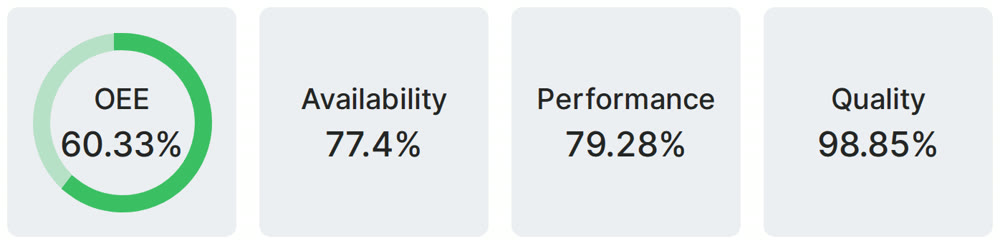
Measured output is the weak spot in many learning curves, because hand counts and timesheets arrive late and rounded. OEE software records counts, run time, stops and scrap per machine and shift automatically, and a light MES ties them to orders and products, so the curve for each product can be plotted from real data. For the cost side of the same numbers, see OEE cost per unit.
How Fabrico fits
Fabrico is a cloud OEE and light MES platform. It shows OEE and losses by machine, line and shift, from the PLC or a Fabrico IoT device, with the reasons operators add on a tablet or phone. That gives you cumulative good units, cycle times and scrap per product and shift: the raw material for a measured learning curve.
On manual stations, AI cameras (an add-on) count output.
Book a demo and see good output per line and shift.
What people ask next
What is the learning curve formula?
The unit formula is Y = A x X to the power b: Y is the hours or cost of unit X, A is the first unit's hours or cost, and b = ln(slope) / ln 2. On an 80% curve b is minus 0.322, so a first unit of $1,000 gives $800 for unit 2 and $640 for unit 4, as in GAO's example.
What does an 80 percent learning curve mean?
Each time cumulative output doubles, the hours or cost per unit fall to 80% of the previous level: unit 2 takes 80% of unit 1, unit 4 takes 80% of unit 2. The percentage is what remains, so 80% saves 20% per doubling and is faster learning than 90%.
What is Wright's law?
Wright's law says cost falls as a power law of cumulative production. T. P. Wright described it for aircraft in 1936. A 2013 PLOS ONE study of 62 technologies found it gave the best cost forecasts, with Moore's law close behind.
How do you calculate a learning curve percentage from your own data?
Take two points of cumulative good units and hours per unit. b = ln(y2 / y1) / ln(x2 / x1) and the learning percentage is 2 to the power b. For example, 19.0 hours at unit 25 and 13.9 hours at unit 100 give b = minus 0.2255 and an 85.5% curve (example data).
What is the difference between unit and cumulative average learning curves?
The unit formulation predicts the cost of each unit. The cumulative average formulation, associated with Wright, predicts the average cost of all units so far. GAO notes the cumulative average shows larger savings over the first few units and suits early production on prototype tooling.
Do production breaks reset the learning curve?
Partly. GAO describes the Anderlohr method, which estimates lost learning across personnel, supervision, production continuity, methods and tooling, and the retrograde method, which restarts production at an earlier unit on the curve. GAO's example of a 6-month break loses 30.9% of learning.
Sources
All sources accessed on 14 November 2026. Dates are the publication dates shown on each page.
- US Government Accountability Office, Cost Estimating and Assessment Guide GAO-20-195G, Appendix VII: unit formulation, undated web edition, accessed 14 November 2026
- Nagy, Farmer, Bui and Trancik, Statistical Basis for Predicting Technological Progress, PLOS ONE 8(2): e52669, February 2013
- Levitt, List and Syverson, Toward an Understanding of Learning by Doing: Evidence from an Automobile Assembly Plant, NBER Working Paper 18017, April 2012
- US Department of Energy, Vehicle Technologies Office, Fact of the Week #1354: EV battery pack costs in 2023 are 90% lower than in 2008, 5 August 2024
- University of Maryland, ENAE 483/788D Principles of Space Systems Design, Lecture 07: Cost Estimation and Engineering Economics, 17 September 2024
- US Bureau of Labor Statistics, Employer Costs for Employee Compensation, Table 4, June 2026, 9 September 2026
Related articles



Latest from our blog



Real Fabrico tiles, sample data.